Manual
General (Main Window)
The following figure shows the resizable Amici main window:
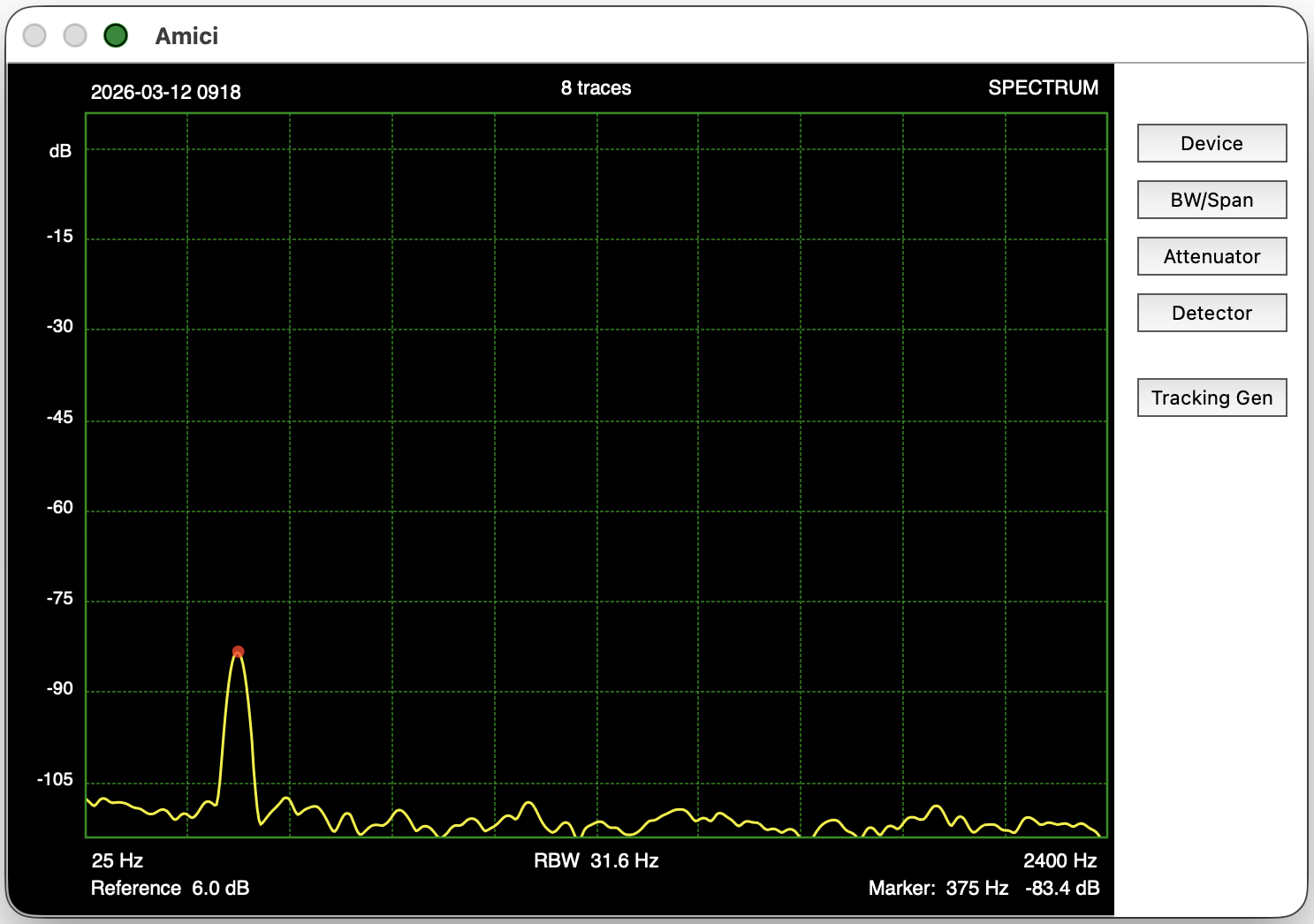
Figure 1 Amici Window
Parameters that are associated with the
spectrum analyzer (e.g., frequency span, resolution bandwidth,
etc.) are located in temporary panels that are opened and closed by the buttons at the right side of the spectrum display. The spectrum trace and surrounding annotations can be saved into a file using
Appearance (Settings Window)
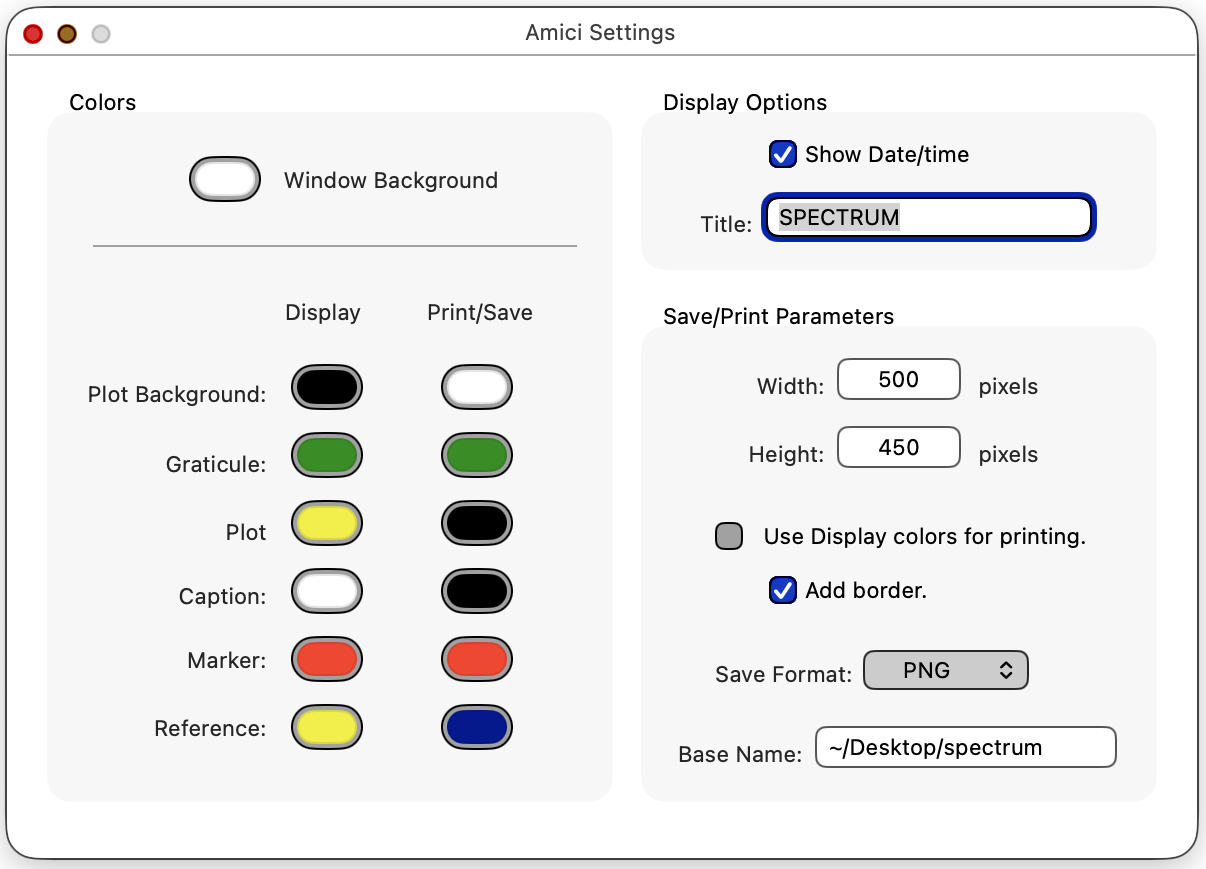
Figure 2 Amici Settings
The box contains color wells that determine the colors for different components of the Amici window. To change the color of a component, click once in the color well and the familiar Color Picker window will be displayed. Do not double click on a color well — because of an idiosyncrasy in Mac OS X, a color well becomes unassociated with the Color Picker when you double click on the well.
The color is the background color of the right side of the window which is under the column of buttons.
There are two sets of colors that can be picked for the actual spectrum display. One set of colors is used for on-screen display, and the second set is use as colors for printing, or when saving a plot to a file. You can print and save with the same colors that appear on the screen by selecting the checkbox that is in the box on the right side of the Amici Settings window.
Printing and Saving Screen Shots (File Menu)
You can send a the spectrum display with annotations directly to a printer by
selecting
You save the display to an
image file using
Figure 3 shows a saved spectrum using the Print/Save colors that are shown in Figure 2 but with the checkbox unselected. The figure also shows the border that is drawn when the checkbox is selected (the border is drawn using the graticule color). The print border is never drawn when display colors are selected for printing. Notice that the default print colors that are shown in Figure 2 are chosen to save ink/toner and quite suitable for black/white printers.
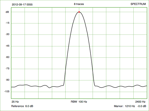
Figure 3 Print/Save Colors (with border)
In the above figure, a Date/time time stamp (YYYY-MM-DD HHMM) is added to the top left of the spectrum display. You can choose not to output the time stamp by unselecting the checkbox in the box of the Settings window. A plot title can also be drawn at the top right of the spectrum display. The title is defined with the text field in the box. This text field can be left empty. The time stamp and plot title shows up in both the display and the print/save versions.
As shown in Figure 2, the size of a saved image is set with the and text fields. This size is independent from the size of the Amici window itself.
The menu allows you to choose between PNG, TIFF or JPEG file formats. When saving a plot, the text field determines where the path name of the written file. Amici will append a date and time and also add a suffix (.png, .tif or .jpg) to the base name for use as the complete file name.
Spectrum Analyzer Input (Device Panel)
Amici takes input from the Macintosh's built-in audio inputs, or from an external USB or FireWire sound card.
The button on the right of the Amici window opens up a panel for chosing sound card parameters. You can close the panel by pressing the button again. Figure 4 shows the opened Device panel.
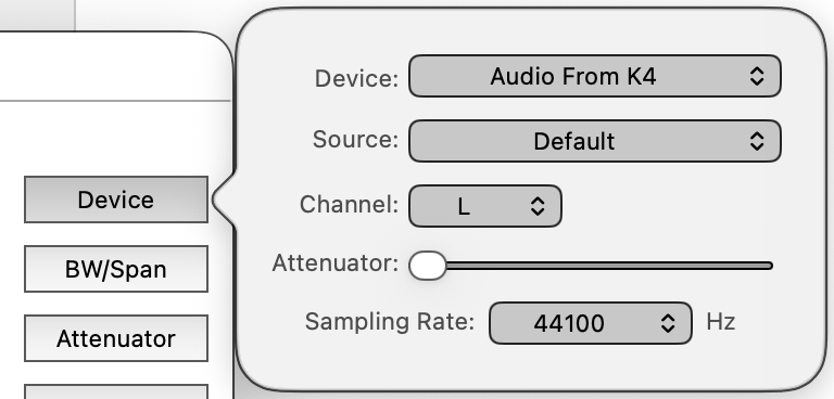
Figure 4 Device Panel
The A/D converter or codec of a sound card can often select between different physical inputs. These inputs are called sources. The codec can only receive input from a single source at a time. For example, the microKeyer II has a single input codec that can either be routed to its microphone input or to its external line input. In the case of the microKeyer, the popup menu is used to select between the two sources. If the sound card has only one source, Amici will show it in the source popup menu as .
Unlike sources, a multi-channel sound cardcan simultaneously access more than one input channel. For stereo devices, the popup menu will show L (left) or R (right) channels. The popup menu for sound cards with more than 2 channels will use an integer number to identify the channel. Except for low level cross-talk, one channel of a codec will not see the input from a different channel. With sound cards that accept stereo phone plugs, the left channel is usually wired to the tip of the phone jack and the right channel is wired to the ring of the jack, with the jack's sleeve acting as a common ground return for the stereo signal.
Sound cards usually support multiple sampling rates. Unless you are measuring signals that are above 20 kHz, it is recommend that you keep the sampling rate at 48000 Hz or lower. Lower sampling rates result in lower processor usage. To measure signals up to N Hertz, you must use a sampling rate that is at least 2N samples/second.
Practically all sound cards are uncalibrated devices. Amici uses the full scale numerical value from the sound card, together with a user settable attenuator field in the panel, to establish the 0 dB reference.
Some sound cards comes with a digitally controlled attenuator that is associated with the slider shown in Figure 4. The sound card attenuator can sometimes be useful for keeping a fixed input signal from saturating the input of a sound card. If an attenuator is not present, Amici will disable the slider (the slider will be grayed out). Be mindful that the slider further alters the reference level of the measured spectrum.
The sound card must never be allowed to clip or saturate. When that happens, the input signal produces nonsensical spectra.
Attenuator and Plot Scale (Attenuator Panel)
Even though sound cards may not have an absolute full scale value, you can still use Amici to make relative readings as long as you keep the device attenuator's slider unchanged. As long as you don't remove an external sound card, Amici will try to maintain the same sound card selection and slider value each time the application is relaunched.
Given a constant input that drives the sound card to full scale, Amici's plot can be adjusted to read 0 dB by setting the text field in the panel opend by the button, seen in Figure 5 below.
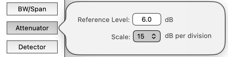
Figure 5: Attenuator Panel
When is set to 0 dB, Amici will display a full scale sinusoid from the sound card, right before the sound card clips, as a 0 dB level on its display.
For most sound cards, this full scale level is an imprecise value, and sound card manufacturers usually do not even dare to publish it in their spec sheets. (Most sound cards have a full scale around 0 dBu.) However, it will likely to also change depending upon the attenuator slider setting, whose position may or may not bear an accurate relationship to the number of dB of actual attenuation. Moreover, some sound cards have a separate microphone and line level input, and the relative gain between them is also an imprecise value.
For this reason, Amici's vertical scale is labeled simply as dB relative to some unspecified value. The actual reference will depend on the sound card's full scale level, the sound card's attenuator setting, and the field that is shown in Figure 5.
As long as you don't switch to a different sound card, don't change the attenuator slider of the sound card (or let another application change it), and don't change the field, you can make meaningful relative readings between devices that you are testing.
You can set the vertical scale of the plot to 1, 2, 3, 6, 10, 15, 20 or 30 dB per division with the popup menu shown in Figure 5. The following two figures show the displays that are set to 15 dB per division and 20 dB per division, respectively:
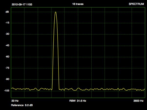
Figure 6 15 dB per Division
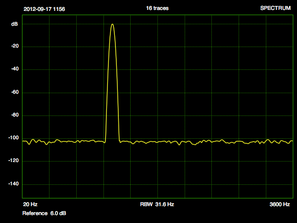
Figure 7 20 dB per Division
The next figure shows the same 20 dB per division scale, but with field in the drawer reduced by 10 dB. Notice that this shifts the entire plot down by 10 dB relative to the grid lines.
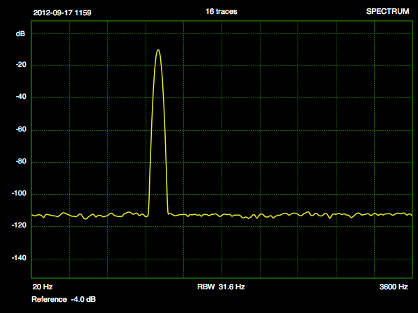
Figure 8 20 dB per
Division with an additional -10 dB change to Reference
Level
If the field or popup menu settings cause the trace to fall either completely above or completely below the display area, Amici draws a gray warning bar at the top or the bottom of the plot, respectively. Figure 9 shows the appearance when the entire trace falls below the display (-75 dB in this case).
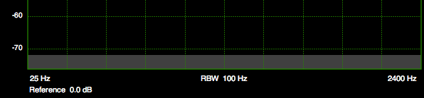
Figure 9 Gray Warning Bar when
trace falls completely below the
Display
Resolution Bandwidth (BW/Span Panel)
While Amici uses the Fast Fourier Transform (FFT) to estimate the power spectrum, it does not depend solely on the FFT to provide the resolution bandwidth that is desired in a spectrum analyzer.
When a 16,384-point FFT is performed on a 48,000
sample/second to produce 8,192 frequency bins, the
resultant bins are separated from one another by 2.929 Hz.
Each bin has a transfer function in the frequency domain
that has the shape of a sin(f)/f function, with the zeros
of the function occurring precisely at the center of bins
other than itself. Each of these FFT bins also has an
equivalent noise bandwidth of 2.929 Hz.
The sin(f)/f transfer function from a raw FFT causes a
signal that is not located precisely at the center of an
FFT bin to also appear at frequency bins that are far away
from the true signal.
Further, it is also desirable for a spectrum analyzer to have selectable noise bandwidth that is different from the natural bandwidth which is determined by the size of an FFT and the sampling rate (i.e., the 2.929 Hz in the example cited above). A noise bandwidth of precisely 1 Hz is especially desirable for the purpose of directly measuring the noise floor of a device and thus being able to directly read out the dynamic range. Noise floors are usually specified in units of dB/Hz.
For these two reasons, Amici applies a calibrated window to the data before performing an FFT on the waveform. To provide a variety of filter skirts, Amici lets you choose between a Hann window, a Blackman window and a Gaussian window.
To create a known bandwidth that is different from the native FFT bin's bandwidth with the Hann and Blackman windows, the support of the window functions are constructed to be narrower than the FFT width. With the Gaussian window, the standard deviation of the Gaussian function provides the bandwidth factor.
Of the three windows available in Amici, the Hann window provides the steepest initial filter skirt, but its sidelobes eventually flare out appreciably.
Although a Hann window produces much lower sidebands than
the sin(x)/x sidebands from a unwindowed FFT, it is still
not useful for making noise floor and IMD measurements that
require a dynamic range of more than about 60 dB.
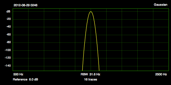
For the same noise bandwidth, the Gaussian window has a wider initial bandwidth than the Hann, but then drops steeply to more than 140 dB at about 3 times the noise bandwidth away from the peak.
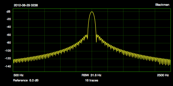
Finally, the Blackman window has a behavior somewhere in between the Hann and the Gaussian.
The following three figures show the behavior of the Hann, Blackman and Gaussian windows, respectively. The window types are shown as the title at the top right hand corner of each figure. All three windows shown here have the same equivalent noise bandwidth of 31.6 Hz, and all windows are plotted to the same scale.
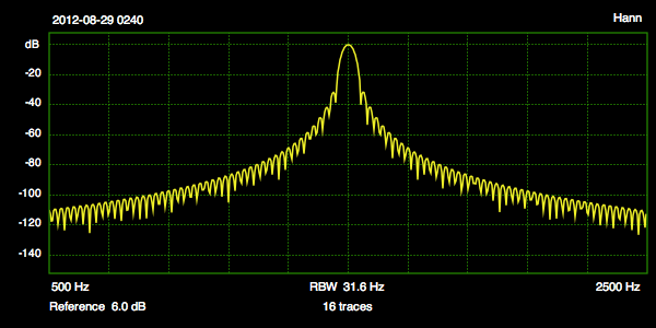
One way to interpret the figures above is that a Hann window is better at separating close spaced tones as long as you do not require a dynamic range that is better than 40 dB.
Amici's Gaussian window, on the other hand is capable of measuring noise floors and IMD in excess of 140 dB (up to the numerical accuracy of single precision floating point FFT) below a reference carrier, but it requires narrower noise bandwidths than the Hann window (and thus more processor cycles due to the need to compute larger FFTs) to resolve two close spaced tones.
The Blackman window is included in Amici to give a solution that sits somewhere between the Hann and the Gaussian.
When processor utilization is not a problem, and if tone separations are greater than 10 times the resolution bandwidth of the filter, it is recommended that you select the Gaussian window.
Figure 10 below shows the and popup menus in the panel opened by the the button.
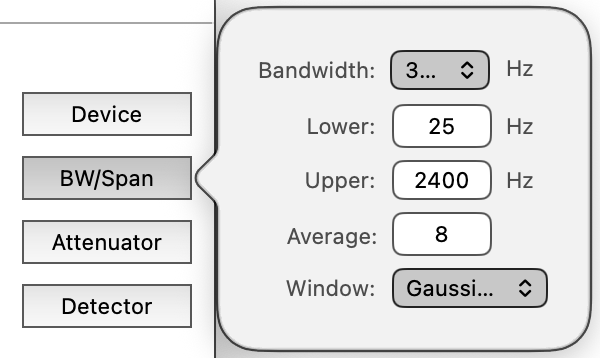
Figure 10 Bandwidth/Span Panel
The menu provides calibrated noise bandwidths of 1 Hz, 3.16 Hz, 10 Hz, 31.6 Hz and 100 Hz (these are equivalent noise bandwidths in 5 dB steps, and accurate to within about 0.1 dB).
The dynamic range of a device can, for example be read directly off the display by using a full scale tone and reading the noise floor using a 1 Hz bandwidth, or it can be measured by using 3.16 Hz bandwidth and adding 5 dB to the result, etc.
The and entry fields let you set the lowest and highest frequencies that are displayed. The upper frequency has to be less than one half the sampling rate i.e., the Nyquist frequency.
Because sound cards do not work at or near DC, the lower frequency is limited by the program to 9 Hz. The specific sound card that you use may require you to use a larger limit for the lower frequency before the measurement is meaningful.
The menu specifies the Resolution Bandwidth (RBW) of the spectrum analyzer. (The Agilent Application Note (150) on RF spectrum analyzers is a good reference to learn spectrum analyzer concepts and terms.)
Unlike many older (RF) spectrum analyzers, Amici does not perform video filtering. To smooth the display noise, Amici instead uses Trace Averaging (see above Agilent application note for the definition of trace averaging). The number of traces that are averaged is set by the field in Figure 10; trace average of 1 is equivalent to no averaging. Each doubling of the number of averaged traces improves the noise of the displayed trace by 3 dB.
The averaged trace is reset each time any Amici parameter that affects the spectrum (e.g., resolution bandwidth) changes. When that happens, the number of averages starts over again with a single trace. Traces are accumulated as each new spectrum arrives, until the number of traces reaches the number of traces that is requested. A per-bin exponential moving average is used to produce the averaged data. The current number of averaged traces is reported above the center of the display.
Detector (Detector Panel)
As mentioned above, the size of the underlying FFT in Amici is determined by the resolution bandwidth and the type of FFT window.
With a Hann window, each FFT bin has to be at least 1.5 times narrower than the desired resolution bandwidth. With a Blackman window, each FFT bin has to be 1.728 times narrower than the desired resolution bandwidth. With the Gaussian window, each FFT bin has to be 1.808 times narrower than the desired resolution bandwidth.
With a typical frequency span and display size, there can also be many FFT bins per horizontal pixel on the display. Typically, this means that many FFT bins will map to a single pixel on the display.
How the multiple FFT bins map to a single pixel that is drawn is determined by the detection method. Amici lets you select between positive peak, negative peak, average, rosenfell and "normal" detection methods from the popup menu in the panel.
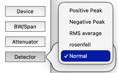
Figure 11 Detector Menu
The Agilent application note has a section which describes various detection modes used in spectrum analyzers. They will only be briefly mentioned here, together with hints on where each detector is useful in the context of audio measurements.
With positive peak detection, the detector picks the largest value from the set of FFT bins that are mapped to a single pixel — this detector is especially useful for accurately measuring the peak power of a narrow tone. It is also useful for accurately determining the higher bound of a passband ripple. The positive peak detector can however misrepresent noise floor measurements by a substantial amount.
With negative peak detection, the detector picks the smallest value from the set of FFT bins that are mapped to a single pixel — this detector not only underestimates the noise floor, it also almost always fail to provide the correct peak value of a narrow tone. It can be useful however, when there is a need to accurately determine of the lower bound of a passband ripple.With average detection, the detector computes the RMS average of the set of FFT bins that are mapped to a single pixel — this is more accurate than both the peak detectors for measuring a mostly constant noise floor of a device. The average detector invariably fails however to provide the correct power of a narrow tone.
Neither of the peak detectors are good in regions where the signal-to-noise ratio is poor, while the average detector fails when the spectrum changes rapidly, including the peak of a narrow tone. For this, there is the rosenfell detector.
The rosenfell detector displays the peak value of the set of FFT bins if the ordered bins are always ascending or always descending. If the FFT bins both rise and fall (thus the name "rosenfell"), the negative peak from the set is used if the resultant pixel is an even pixel. The positive peak from the set of FFT bins is used if the resultant bin is an odd pixel. The rosenfell detector will therefore always give the correct peak power of a narrow tone, although it can sometimes draw the peak of a tone one pixel to the right if the tone peak happens to fall on an even pixel. I.e., the rosenfell can produce correct peak values, although the location of the peak can be off by one pixel in frequency, while not over-estimating the noise floor (the human eye can average out the positive and negative peaks in the noise).
Amici uses a modified rosenfell detector as its "normal" detector. Instead of using the negative peak as an even pixel of the rosenfell detector, the normal detector in Amici uses the RMS average as the even pixel. This provides a slightly a better visual estimate of the noise floor than the standard rosenfell detector.Many RF spectrum analyzers use the standard rosenfell as their "normal" detector. If you want to use the rosenfell detector in Amici, you need to select it explicitly instead of using the "normal" detector.
Marker (Display Context Menu)
In Amici, a marker is placed on a spectrum trace by using the contextual menu of a right mouse click inside the trace display area.
First, make sure the Amici window is active. If you are not certain, you can safely click on the title bar of the window to activate Amici. If the mouse cursor is not already an arrow cursor, activating Amici should turn it into an arrow cursor.
Position the pointed end of the arrow cursor at or near the location in the spectrum trace where you wish to set a marker. Then hold down the right mouse button (if your mouse does not have a right button, you can first hold down the keyboard control key before holding down the normal mouse button). You will see a contextual menu like the one that is shown in Figure 12:
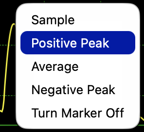
Figure 12 Marker Contextual Menu
Once the contextual menu is visible, you can move the cursor to one of the menu items and release the mouse button.
The menu item places the marker at a sample on the curve that is nearest to where you had initially held the mouse button down.
A dot is drawn on the display to indicate the sample location that is picked. The color (default color is red) of the dot is defined by the color in the Settings window. The frequency and power level of the marker is shown at the lower right of the display (-66.7 dB at 1521 Hz in Figure 13).
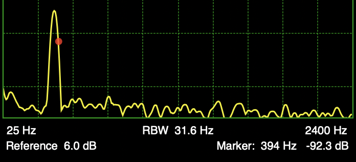
Figure 13 Marker Location and Value
Please note that when the curve is steep, Amici may not pick the closest point on the curve to locate the marker. The marker is instead placed at the closest detected point.
When a new spectrum trace arrives after a sample marker has been placed, the marker keeps the same frequency, but moves to the new measured power level if that has changed. The marker's textual information is also updated.
An existing marker is removed when a new marker is selected. You can remove a marker completely by choosing the menu item in the contextual menu.
The marker places the marker at the closest positive peak on the curve to the selected point. When a new spectrum trace arrives, Amici will update the location of the peak.
The marker places the marker at the closest negative dip on the curve to the selected point and will similarly be updated when a new trace arrives.
The marker first locates the closest point on the curve and then computes the average of the trace surrounding that point. Amici takes the average power for a frequency interval that is approximately equal to 5% of the total displayed frequency span and centered at the selected point, resulting in an RMS measurement near the selected point. Amici displays the averaged span with a translucent bar (whose vertical location is the average power), as shown in Figure 14:
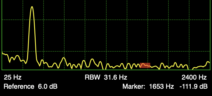
Figure 14 Average Marker Location and Value
The selected frequency (midpoint of the averages) and average power level are listed at the lower right of the Amici display, as shown in Figures 14.
Tracking Generator (Tracking Gen Panel)
Amici includes a tracking generator for measuring the transfer function of filters and devices.
It is highly recommended that you first use a wider bandwidth such as 31.6 Hz for initial measurements, and reduce the bandwidth only when needed.
To use the tracking generator, feed the generator's output sound card to the input of device under test (DUT), and connect the output of the DUT back to the input of the Amici.
Figure 15 shows the panel. Like Amici's input, there is a set of parameters for the tracking generator's sound card. You need not use the output codec from the input sound card — but be aware that there could be slight difference in actual sampling rates between two different sound cards unless one of then is synched with the other. This is not generally a problem when you set the Amici bandwidth to 10 Hz and above. You can also use the Mac OS X's Audio MIDI Setup utility to combine sound cards into an aggregate device that share the same sampling rate clock — see this Apple technical note.
![]()
Figure 15 Tracking Generator Panel
To place Amici into tracking generator mode, switch the radio buttons in the drawer to . This will erase any previous spectrum analyzer trace from the display. Click the button to start the tracking generator. The Start button's label will now read . You can stop the tracking generator and restart the generator from the beginning by toggling the Start/Stop button.
Amici will start the tracking generator at a frequency that is slightly lower than the lower of the display's frequency span. Because of that, nothing may show up for a little while. Amici will initially display a set of gray spinning discs at the center of the display to indicate activity. The spinning discs are removed a short time after the spectrum trace appears.
A vertical gray line shows the progress of the tracking generator as it sweeps the spectrum.
Figure 16 shows both the set of spinning discs which appear at the beginning of a tracking generator sweep and the vertical progress line.
![]()
Figure 16: Spinning discs and
progress line of the Tracking Generator display.
The tracking generator stops at the end of the trace and the Start/Stop button label shows Start again. Trace averaging is turned also off when Amici is in the tracking generator mode.
If you restart the tracking generator after a trace has completed, Amici will replace the samples on the old trace in the display with the new trace without erasing samples from the old trace that the tracking generator has not yet reached in the subsequent pass. (To erase the old trace, you can quickly toggle the state of the tracking generator between Off and On.) The vertical gray progress line will show where the new trace ends and where the old trace begins.
Just like the spectrum analyzer mode, Amici allows you to place a marker on a tracking generator trace. If you ask for a positive peak or a negative peak and the tracking generator has not yet reached the neighborhood peak, the marker will follow the tracking generator's frequency until such peck is reached. For example, if you ask for a negative peak near the frequency the tracking generator is on, and the measured power is still decreasing, the marker location will follow the tracking generator.
Figure 17 shows the tracking generator output of a second order lowpass RLC filter with a marker set for the positive peak.
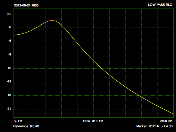
Figure 17: Lowpass RLC
filter
Reference Spectrum (Reference menu)
In addition to the ability to send the display directly to a printer, or to a PDF file, or to save the display as an image file (see Printing and Saving Screen Shots section above), Amici can also save the current spectrum trace to a data file that can subsequently be used as a reference plot.
Figure 18 shows the
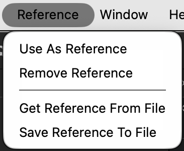
Figure 18: Amici Reference Menu
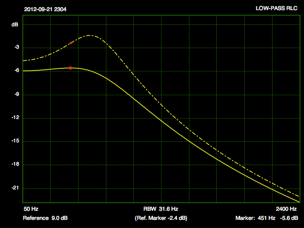
Figure 19: Spectrum (from
tracking filter) with Reference
You can export an existing
trace as an XML format file by selecting
As seen in Figure 19 above, when you set a marker on the current trace, it will also report the value of the reference at the same frequency. The reference marker value is shown at the bottom center of the display.