Terminations
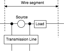
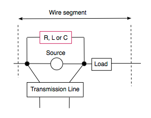
The diagram below shows the relationship between a source, a load and a transmission line when they are placed in the same segment of a wire in NEC:
impedanceTermination( element, R, X ) impedanceTermination places an impedance R+iX at the center of the wire element, such that it terminates (shunts) both a source at that segment and a transmission line at that segment of the wire, as shown below: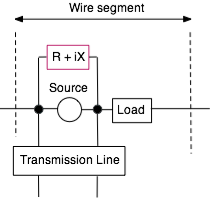
lumpedParallelTermination( element, R, L, C ) lumpedParallelTermination places a resistor, inductor and capacitor at the center of the wire element, such that it terminates (shunts) both a source at that segment and a transmission line at that segment of the wire, as shown below: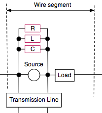
lumpedSeriesTermination( element, R, L, C ) lumpedSeriesTermination places a series connected resistor, inductor and capacitor at the center of the wire element, such that the combination terminates (shunts) both a source at that segment and a transmission line at that segment of the wire, as shown below: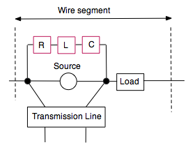
resistiveTermination( element, R )

			capacitiveTermination( element, C )

inductiveTermination( element, L ) - The above place an individual resistor, inductor or capacitor at the center of the wire element, such that the combination terminates (shunts) both a source at that segment and a transmission line at that segment of the wire, as shown below:
Physical Coax and Twin-lead Transmission Lines.
The NC
transmissionLine function generates a NEC TL card to insert a transmission line between two wire elements. While you can model the characteristic impedance and velocity factor, a TL card does not model DC losses, skin effect losses or dielectric losses. The TL card also does not physically exist, and only models voltage and currents at the ends of the line.Just as wires in NC have the type element, a coax or twin-lead in NC has a type coaxtype. And, like wire elements, you can assign a coaxtype variable to another. Some examples of how coaxtype variables and constants can be used are shown here:
				element e1, e2 ;

				coaxtype mycoax ;


				e1 = wire( 0, -5, 12, 0, 5, 12, 0.01, 21 ) ;

				e2 = wire( 4, -5, 12, 4, 5, 12, 0.01, 21 ) ;

				mycoax = RG58 ; // RG58 is a built-in constant

				coax( e1, e2, RG58 ) ;

				coax( e1, e2, mycoax ) ; // this statement does the same thing as the previous statement
The next two sections describe built-in coaxtype constants for some common coax cables and window lines. These constants can be used anywhere a coaxtype variable can be used.
Coax Cable Types
The following are (case sensitive) manifest constants for coax cables in NC.
| coaxtype | Nom. Zo | Velocity Factor | Manufacturer Type |
|---|---|---|---|
| RG6 | 75 Ω | 0.66 | Belden 8215 |
| RG6hdtv | 75 Ω | 0.83 | Belden 7915A |
| RG6catv | 75 Ω | 0.83 | Belden 9116 |
| RG8 | 52 Ω | 0.66 | Belden 8237 |
| RG8foam | 50 Ω | 0.82 | Belden 9914 |
| RG8X | 50 Ω | 0.82 | Belden 9258 |
| RG11 | 76 Ω | 0.66 | Belden 9212 |
| RG11foam | 75 Ω | 0.84 | Belden 8213 |
| RG58 | 51.5 Ω | 0.66 | Belden 8240 |
| RG58foam | 53.5 Ω | 0.73 | Belden 8219 |
| RG59 | 75 Ω | 0.66 | Belden 8241 |
| RG59foam | 75 Ω | 0.78 | Belden 8212 |
| RG62 | 90 Ω | 0.84 | Belden 9269 |
| RG174 | 50 Ω | 0.66 | Belden 8216 |
| RG213 | 50 Ω | 0.66 | Belden 8267 |
| LMR100 | 50 Ω | 0.66 | Times Microwave LMR®-100A |
| LMR200 | 50 Ω | 0.83 | Times Microwave LMR®-200 |
| LMR240 | 50 Ω | 0.84 | Times Microwave LMR®-240 |
| LMR300 | 50 Ω | 0.85 | Times Microwave LMR®-300 |
| LMR400 | 50 Ω | 0.85 | Times Microwave LMR®-400 |
| LMR600 | 50 Ω | 0.87 | Times Microwave LMR®-600 |
| LMR900 | 50 Ω | 0.87 | Times Microwave LMR®-900 |
| BuryFLEX | 50 Ω | 0.82 | Davis RF Bury-FLEX™ |
| LDF4 | 50 Ω | 0.88 | Andrew LDF4-50A Heliax® |
| LDF5 | 50 Ω | 0.89 | Andrew LDF5-50 Heliax® |
| LDF6 | 50 Ω | 0.89 | Andrew LDF6-50 Heliax® |
Twin Lead Types
The following are (case sensitive) manifest constants for twin-lead cables which are defined in NC.
| coaxtype | Zo | Velocity Factor | Wire Gauge | Nom. Zo |
|---|---|---|---|---|
| Generic450ohm | 450 Ω | 0.91 | ||
| Generic600ohm | 600 Ω | 0.97 | ||
| Wireman551 | 400 Ω | 0.902 | 18 AWG solid | 450 Ω |
| Wireman551wet | 390 Ω | 0.864 | 18 AWG solid | 450 Ω |
| Wireman552 | 380 Ω | 0.918 | 16 AWG stranded | 450 Ω |
| Wireman552wet | 365 Ω | 0.883 | 16 AWG stranded | 450 Ω |
| Wireman553 | 395 Ω | 0.902 | 18 AWG stranded | 450 Ω |
| Wireman553wet | 380 Ω | 0.869 | 18 AWG stranded | 450 Ω |
| Wireman554 | 360 Ω | 0.93 | 14 AWG stranded | 440 Ω |
| Wireman554wet | 350 Ω | 0.87 | 14 AWG stranded | 440 Ω |
| JSC1318 | 380 Ω | 0.89 | 16 AWG stranded | 450 Ω |
Defining other coaxtypes
You can define your own coaxtype by calling and assigning the
coaxModel function to a coaxtype variable:coaxModel( Zo, velocityFactor, k0, k1, k2, shieldDiameter, overallDiameter, jacketPermittivity )Zo and velocityFactor are the known characteristic impedance and velocity factor of the cable,k0 accounts for the DC resistance/length of the conductors,k1 accounts for the high frequency resistance/length of the conductors due to skin effect,k2 is the dielectric loss,shieldDiameter is the diameter (in meters) of the coax shield,overallDiameter is the overall diameter of the coax cable (including the outer jacket),jacketPermittivity is the relative permittivity of jacket material (about 3.2 for PVC and 2.25 for Polyethylene)The shield diameter, overall diameter and jacket material values can be obtained from the manufacturer's specifications. The shield diameter is only used in NC functions that model the shield. When used with functions that ignores the shield, the shieldDiameter can be set to zero.
If the overall diameter is equal to or less than the shield diameter, the shield is assumed to be in free space, otherwise a Yurkov insulation approximation is applied to the wire which models the shield.
Sources other than AC6LA may approximate the frequency-independent DC loss (k0) by curve fitting it into the skin effect loss (k1). If that is the case, set the k0 term to zero. Separating k0 and k1 provides a better approximation of cable characteristics below about 10 MHz.
Note that the transmission line loss constants
k0, k1 and k2 are expressed in length units of meters. AC6LA's Transmission Line Details expresses lengths in units of 100 feet. The k0, k1 and k2 constants from AC6LA's program must be multiplied by 0.0328084 (the number of feet in 1 meter, divided by 100) when used in the coaxModel function.For example, the Belden 8216 (RG-174) can be defined and used to create a cable that connects two wire elements as follows:
			element e ;

			element e1, e2 ;

			coaxtype myRG174 ;


			e1 = wire( 0, -5, 12, 0, 5, 12, 0.01, 21 ) ;

			e2 = wire( 4, -5, 12, 4, 5, 12, 0.01, 21 ) ;


			myRG174 = coaxModel( 50, 0.66, 0.0707, 0.0255, 0.2852e-3, 2.11e-3, 2.8e-3, 3.18 ) ;

			coax( e1, e2, myRG174 ) ;
Some other examples are:
			coaxModel( 50, 1.00, 0, 0, 0, 5.7e-3, 0, 0 ) // lossless 50 ohm coax with velocity factor 1.0

			coaxModel( 50, 0.80, 0, 0, 0, 5.7e-3, 0, 0 ) // lossless 50 ohm coax with velocity factor 0.8
coaxModel( 52, 0.66, 0, 0, 0, 7.8e-3, 0, 0 ) // lossless "RG-8" coax
coaxModel( 52, 0.82, 8.5e-4, 6.09e-3, 4.45e-5, 7.8e-3, 10.3e-3, 3.18 ) // "RG-8" coax with velocity factor 0.82
A twin-lead can similarly be defined with:
twinleadModel( Zo, velocityFactor, k0, k1, k2, wireSeparation, insulationDiameter, insulationPermittivity )wireSeparation is the separation (in meters) between the two wires,insulationDiameter is the model of the diameter of the insulation around each wire (includes connected portions of a window line),insulationPermittivity is the model of the permittivity of the insulation.Transmission Line Models
NC uses the admittance matrix of an NT (network) card in NEC to model the transmission line characteristics of a physical cable.
While the models here take into account transmission line properties such as the velocity factor and losses in a coax cable, they do not account for common mode currents. For models that roughly approximate shield currents, use the NC functions in the Coax Models With Shield section below.
The transmission line model uses estimates for the DC resistance/length of the conductors (k0), the high frequency resistance/length of the conductors due to skin effect (k1), the dielectric loss (k2), the real part of the characteristic impedance (Zo), the velocity factor and the frequency.
RLGC values are first computed from the transmission line parameters. Next, the complex propagation constant (gamma) and the complex admittance (Yo) are computed from the lumped constants R, L, G and C.
Finally, using the lossy transmission line equation, y11 and y12 of the passive two-port NT network are computed from gamma, Yo and the physical length of the cable. y22 for the NT card is set to be the same as y11.
A no-zero input admittance that appears in a
terminatedCoax call is added to the y11r and y11i parameters of the NT card. An output admittance is similarly added to the y22r and y22i parameters of the NT card. A crossed wire is implemented by negating the y12r and y12i parameters of the NT card.Because the frequency is needed to determine the y parameters of the NT card, NC defers computation of the y matrix until after the frequency is known (from the
setFrequency, addFrequency or frequencySweep functions). When there are multiple frequencies, a different NT card is generated for each FR (frequency) card.
NC Functions for creating Coax Cables
coax( element1, element2, type )- The
coax function places a coax cable between the middle of wire element1 and the middle of wire element2. The argument "type" is a coaxtype constant or variable. For example, coax( element1, element2, RG8 ) places an RG-8 cable between the centers of wire element1 and wire element2.The center conductor of the coax cable is the middle of the center segment of a wire that has odd number of segments. If the wire has an even number of segments, the "center" is segment number (N+1)/2 (rounded down) where N is the number of segments. The polarity is such that the "shield" of a coax electrically attaches to the junction of the central segment and the next segment that is closer to the second end of the wire (the second end is the second set of (x,y,z) coordinates when the wire is defined.
crossedCoax( element1, element2, type )- The
crossedCoax function includes a 180 degree phase reversal. terminatedCoax( element1, element2, type, y1r, y1i, y2r, y2i )crossedTerminatedCoax( element1, element2, type, y1r, y1i, y2r, y2i )- A
terminatedCoax includes an admittance y1r+i.y1i (in mhos) at the first (element1) end of the transmission line, and an admittance y2r+i.y2i on the other (element2) end. It allows you to conveniently short out the end of a coax cable when used as a stub.
terminatedCoax( element1, element2, type, 0, 0, 1.0e6, 0 ) effectively shorts out the element2 end of the coax, while terminatedCoax( element1, element2, type, 0, 0, 0, 0 ) is the same as calling the coax function above.crossedTerminatedCoax has a 180 degree phase reversal on one end.The physical coax model consists of two components. Like the unshielded coax case above, one component models the transmission line aspect of the coax with an NT card, and the second component models the shield.
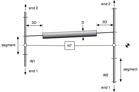
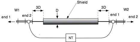
NEC inserts sources, networks and transmission lines at the middle of a wire segment. The middle of the center segment of the each wire is shown above as an open circle.
On the other hand, NEC connects wires at the end of segments. For this reason, NEC cannot attach both the center of the shield and the center of the inner conductor of the coax to the same precise location on a wire.
As shown in the diagram above, the NT card is inserted between the middle of W1 and the middle of W2, while the outer shield of the coax is modeled as a fat wire with diameter D that is connected to one of the ends of the central segment of each wire. The structure length of the shield is 6D shorter than the connecting distance between W1 and W2. A tapered wire connects the shortened shield to W1 and W2. The model becomes more accurate as the segment sizes of W1 and W2 are made smaller, since the distance from the NT connections and the shield connects become smaller.
By convention, cocoaNEC connects the shield to the end of a wire segment that is closer to end 2 of W1 and W2. end 2 is the second set of coordinates that is used to define a wire. If a crossed coax connection is requested, in addition to a phase reversal of the NT card, the coax shield is connected to the end of a segment that is closer to end 1 of W2.
NC Functions for creating Coax Cables With Shields
The function arguments for the coax models which include shields are the same as the function arguments for the functions where shields are not generated:.
coaxWithShield( element1, element2, type )

		crossedCoaxWithShield( element1, element2, type )

		terminatedCoaxWithShield( element1, element2, type, y1r, y1i, y2r, y2i )

		crossedTerminatedCoaxWithShield( element1, element2, type, y1r, y1i, y2r, y2i )
These functions should not be used with twin-lead coaxtypes.
The following is an example of using the coaxWithShield function to model the common mode currents on the shield of a coax cable that feeds a horizontal dipole:
model( "common mode radiation example" )
{
element wLeft, w1, wRight, w2 ;
real span, height, d ;
span = 5.2 ;
height = 5.6 ;
d = 0.1 ;
// dipole
wLeft = wire( -span, 0, height, -d, 0, height, #14, 21 ) ;
w1 = wire( -d, 0, height, d, 0, height, #14, 5 ) ;
wRight = wire( d, 0, height, span, 0, height, #14, 21 ) ;
// coax end
w2 = wire( -d, 0, 0.5, d, 0, 0.5, #14, 5 ) ;
voltageFeed( w2, 1, 0 ) ;
coaxWithShield( w1, w2, RG8 ) ;
freespace() ;
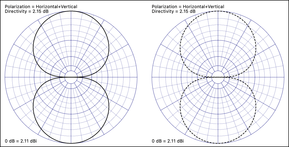
} The azimuth radiation patterns below are produced by the example code above. The following figure shows the effect of using the
coax function instead of the coaxWithShield function. Horizontal polarization is shown in solid lines, and vertical polarization is shown in dashed lines. 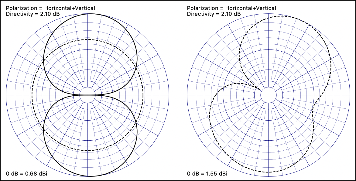
Instead of connecting the coax at the middle of a wire, the following functions allows you to choose to connect to the middle or to either end of a wire. Connecting to the ends of wires lets you connect the coax axially, as shown below (connecting end2 of wire W1 to end1 of wire W2):
endFedCoax( element1, end1, element2, end2, type )endFedTerminatedCoax( element1, end1, element2, end2, type, y1r, y1i, y2r, y2i )end1 and end2 are integer values that are either 0, 1, 2, 10, 11 or 12. The least significant digit of end1 or end2 specifies the location of the wire the coax cable is connected to.
A location value of 0 connects the coax to the middle of the wire as in earlier coax functions. A value of 1 for
end1 connects the coax to the start of wire element1. A value of 2 for end1 connects the coax to the end of wire element1 (the start of a wire is the first set of coordinates when a wire is created).Likewise, the least significant digit of
end2 selects whether you want to connect the coax to the middle or either end of element2.The tens digit of the end1 and end2 flags indicate if the shield is to be left disconnected (this lets you easily model axial stubs that are found in antennas that uses the shield of a cable as radiating elements). If a non-zero flag value is seen, the shield at that end of the coax cable is left unconnected to the wire, i.e., the short wire of length 3D in the above diagram will be left out.
If the shield flag exists on both end1 and end2, the entire shield wire in the model is also left out.
When endFed coax functions are used with twin-lead coaxtypes, the shield flags are set automatically (twin leads have no shield).
Insulated Wire Extensions
See Antenna Modeling Notes, Volume 4, Chapter 83 for a discussion of Insulated Sheath models.
cocoaNEC provides alternate ways to represent an insulated wire other than the IS (insulated sheath) card in NEC-4 and for users of NEC-2, where the IS card is not implemented.
The following NC function implements the approximation by Alexander Yurkov (RA9MB) with 0.92 as the velocity factor for the Yurkov insulation.
yurkovInsulate( element, permittivity, radius, velocityFactor )yurkovInsulate is similar to the insulate() function in NC, but always uses the Yurkov approximation even when running with NEC-4.cebikInsulate( element, permittivity, radius )- The Cebik approximation for insulated wires is similar to the Yurkov approximation above, but uses L. B. Cebik's approximation.
keepDataBetweenModelRuns( state )- Each time a model is executed from a control function by using runModel, the result from a previous run in the Smith Chart and Scalar Plot outputs are replaced by new data. This function plots new feed points without erasing the previous feed points. Sample code
OCF sweep.nc in the Examples folder illustrates plotting a sequence of feed point impedances of an off-center fed dipole as the feed point location is moved.